Insurance Premium Prediction Analysis
Problem description
- To do the EDA to find the important factors affecting the premium price.
- Based on the user input, need to predict the premium price.
Importing Python Libraries
import numpy as np
import pandas as pd
import matplotlib.pyplot as plt
import seaborn as sns
import plotly.express as px
import statsmodels.api as sm
from scipy.stats import stats, shapiro, boxcox, mannwhitneyu, chi2_contingency
from sklearn.model_selection import train_test_split, KFold, cross_val_score
from sklearn.preprocessing import StandardScaler, LabelEncoder
from sklearn.linear_model import LinearRegression, Ridge, Lasso
from sklearn.ensemble import RandomForestRegressor
from sklearn.metrics import mean_squared_error, mean_absolute_error, r2_score
import xgboost as xgb
import lightgbm as lgb
import warnings
warnings.filterwarnings('ignore')
Loading the Dataset
df = pd.read_csv("insurance.csv")
Preliminary Analysis
df.shape
df.head()
df.info()
df.describe()
df.isnull().sum()
- It is clear that there are no missing values in the dataset.
Outlier Detection
columns = df.select_dtypes(include='number')
for col in columns:
    q1, q3 = df[col].quantile([0.25, 0.75])
    iqr = q3 - q1
    lower, upper = q1 - 1.5 * iqr, q3 + 1.5 * iqr
    count = ((df[col] < lower) | (df[col] > upper)).sum()
    print(f"{col}: {count} outliers")
for col in columns:
    q1, q3 = df[col].quantile([0.25, 0.75])
    iqr = q3 - q1
    lower, upper = q1 - 1.5 * iqr, q3 + 1.5 * iqr
    outliers = df[(df[col] < lower) | (df[col] > upper)]
    print(f"Outliers in {col}:\n{outliers}\n{'-'*100}")
out_cols = ['AnyTransplants', 'AnyChronicDiseases', 'Weight', 'KnownAllergies', 'HistoryOfCancerInFamily', 'NumberOfMajorSurgeries', 'PremiumPrice']
for cols in out_cols:
    print('_'*100)
    print(df[cols].value_counts())
- From the above analysis, these outliers should to be removed.
Visual Analysis
Univariate Analysis
# Creating new feature BMI for the better analysis
df['BMI'] = round(df['Weight'] / ((df['Height'])/100)**2, 2)

# Creating BMI categories bin based on standard classifications
df['BMI_Category'] = pd.cut(df['BMI'],
                           bins=[0, 18.5, 25, 30, float('inf')],
                           labels=['Underweight', 'Normal', 'Overweight', 'Obese'])

df['BMI_Category'].value_counts()
clmns = ['Age', 'PremiumPrice', 'BMI']

for cols in clmns:
    plt.figure(figsize=(12, 10))
    sns.histplot(data=df, x=cols, kde=True, bins=30, color='blue')
    plt.title(f"{cols} Distribution")
    plt.show()
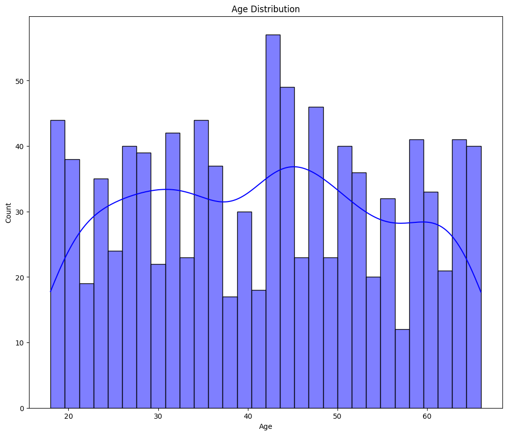
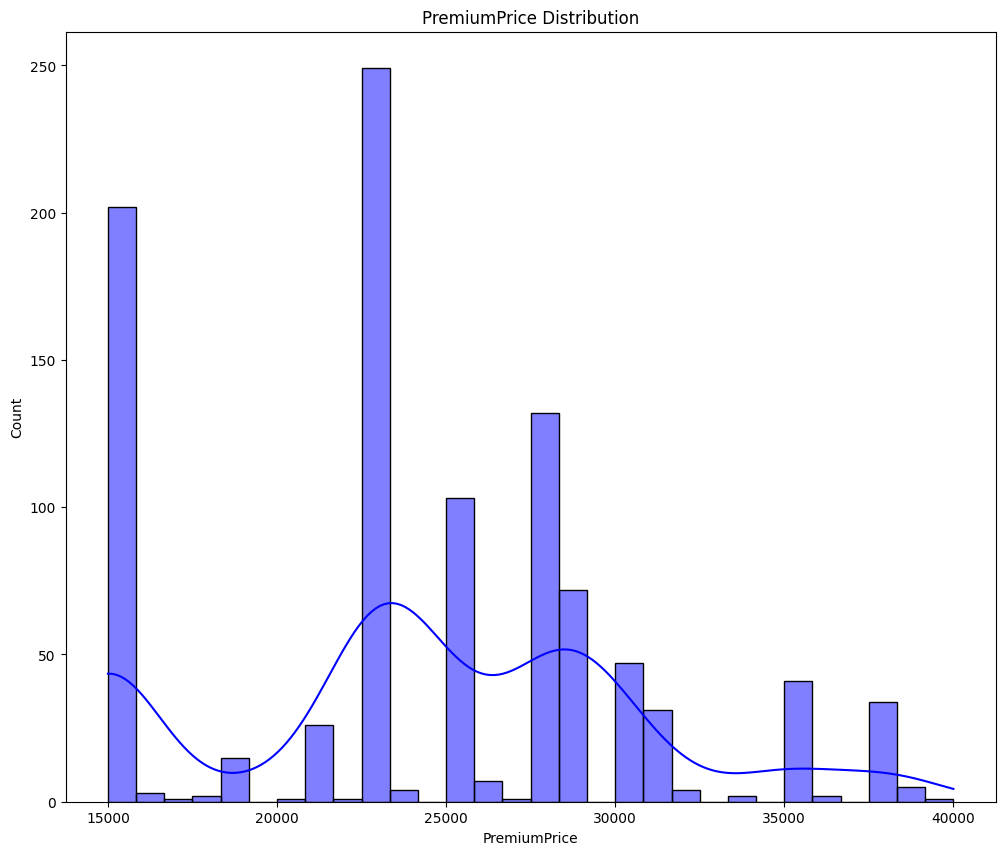
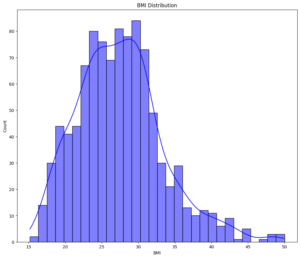
- From the above graphs - Age and Premium Price are not normally distributed.
- BMI seems normally distributed but slightly right skewed.
- We will use statistical test to check and confirm the normality.
Multi-variate Analysis
fig = px.scatter(df, x='Age', y='PremiumPrice',
                 title='Premium Price by Age and BMI',
                 color='BMI_Category', color_continuous_scale='Viridis')
fig.update_layout(title_x=0.5)
fig.show()
💡 Older - Obese and overweight people are got higher premium price.
💡 Younger - Normal and underweight people are got lower premium price.
cat_cols = ['Diabetes', 'BloodPressureProblems', 'AnyTransplants', 'AnyChronicDiseases', 'KnownAllergies', 'HistoryOfCancerInFamily']
for cols in cat_cols:
    df[cols] = df[cols].astype(str)
    fig = px.scatter(df, x='Age', y='PremiumPrice', color=cols, title=f'Premium Price by Age and {cols}',
                        color_discrete_map={"0": 'red', "1": 'green'})
    fig.update_layout(title_x=0.5)
    fig.show()
- Those people have gone for the transplant, got the higher premium price.
fig = px.scatter(df, x='Age', y='PremiumPrice', size="NumberOfMajorSurgeries", color="NumberOfMajorSurgeries",
                 title='Premium Price by Age and Number of Major Surgeries', color_discrete_map={0: 'red', 1: 'green', 2: "blue", 3: "yellow"})
fig.update_layout(title_x=0.5)
fig.show()
- People who are more than 60years old have gone through 3 major surgeries. And their premium prices are same 28K.
- For 2 major surgeries, around the age of 50 to 60 years old, their premium amount is also same 28K.
Statistical Analysis
Pearson = df[['Age', 'PremiumPrice', "BMI", "NumberOfMajorSurgeries"]].corr('pearson')
Spearman = df[['Age', 'PremiumPrice', "BMI", "NumberOfMajorSurgeries"]].corr('spearman')

fig = px.imshow(Pearson,
            text_auto='.2f',
            color_continuous_scale='RdYlBu_r',
            title='Pearson Correlation Heatmap',
            aspect='auto')
fig.update_layout(title_x=0.5, width=800, height=600)
fig.show()

fig = px.imshow(Spearman,
                text_auto='.2f',
                color_continuous_scale='RdYlBu_r',
                title='Spearman Correlation Heatmap',
                aspect='auto')
fig.update_layout(title_x=0.5, width=800, height=600)
fig.show()
- Age and premium price are highly co-related.
num_cols = df.select_dtypes(include=['number']).columns.tolist()

n_cols = len(num_cols)
n_rows = (n_cols + 2) // 3

fig, axes = plt.subplots(n_rows, 3, figsize=(15, 5*n_rows))
axes = axes.ravel()

for i, col in enumerate(num_cols):
    sm.qqplot(df[col], line='45', ax=axes[i])
    axes[i].set_title(f'Q-Q Plot of {col}')

for j in range(i+1, len(axes)):
    axes[j].set_visible(False)

plt.tight_layout()
plt.show()
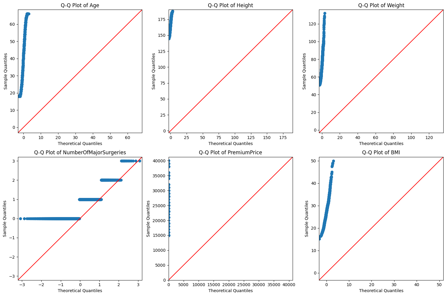
for cols in num_cols:
    stat, p_value = shapiro(df[cols])
    print(f'Shapiro-Wilk Test for {cols}: Statistic={stat:.4f}, p-value={p_value:.4f}')

    if p_value > 0.05:
        print('Data appears to be normally distributed')
    else:
        print('Data does not appear to be normally distributed')
    print('_'*100)
- From the above 2 tests, the premium price, age, height, weight and BMI are not normally distributed.
# Log transform
for cols in num_cols:
    df[f'{cols}_log'] = np.log(df[cols])

num_cols_log = ["PremiumPrice_log", "Age_log", "Height_log", "Weight_log", "BMI_log"]

for cols in num_cols_log:
    stat, p_value = shapiro(df[cols])
    print(f'Shapiro-Wilk Test for {cols}: Statistic={stat:.4f}, p-value={p_value:.4f}')

    if p_value > 0.05:
        print('Data appears to be normally distributed')
    else:
        print('Data does not appear to be normally distributed')
    print('_'*100)
- After the log transform the data are still not normally distributed. So we will use the original data without transformation.
# Since the data is not normally distributed, we will use non-parametric tests for the statistical Analysis

# Instead of t-test, we use Mann-Whitney U test

cols_grps = ['Diabetes', 'BloodPressureProblems', 'AnyTransplants', 'AnyChronicDiseases', 'KnownAllergies', 'HistoryOfCancerInFamily']

for cols in cols_grps:
    group1 = df[df[cols] == 0]['PremiumPrice']
    group2 = df[df[cols] == 1]['PremiumPrice']

    statistic, p_value = mannwhitneyu(group1, group2, alternative='two-sided')
    print(f'{cols} vs Premium price')
    print(f'  Mann-Whitney U Test: p-value = {p_value:.4f}')

    if p_value < 0.05:
        print(f'  Significant difference in Premium Price by {cols}')
    else:
        print(f'  No significant difference in Premium Price by {cols}')
    print('_' * 100)
- From the statistical test, except the Known Allergies all other Diabetes, Blood pressure, Transplants, Chronic diseases and History of Cancer in Family have significant difference in Premium Price.
df['AgeGroup'] = pd.cut(df['Age'], bins=[0,30,50,100], labels=['Young','Middle','Senior'])

def grp (feature, df):
    groups_age = [group['PremiumPrice'].values for name, group in df.groupby(feature)]
    stat, p = stats.kruskal(*groups_age)
    print(f"Kruskal-Wallis Test for {feature}: H-stat =", stat, " p-value =", p)

    if p<0.05:
        print(f'Atleast one of the {feature} has a different Premium Median')
    else:
        print('No difference')

grp ('AgeGroup', df)
grp ('BMI_Category', df)
- From the above analysis, both BMI and Age different groups have significant impact on the premium price.
df['PremiumPrice_Category'] = pd.cut(df['PremiumPrice'],
                                    bins=3,
                                    labels=['Low', 'Medium', 'High'])

cat_cols = ['Diabetes', 'BloodPressureProblems', 'AnyTransplants', 'AnyChronicDiseases', 'KnownAllergies',
                'HistoryOfCancerInFamily', 'BMI_Category', 'AgeGroup']

for cols in cat_cols:
    contingency_table = pd.crosstab(df[cols], df['PremiumPrice_Category'])
    chi2, p_value, dof, expected = chi2_contingency(contingency_table)

    print(f'Chi-Square Test: {cols} vs Premium Price Category')
    print(f'Chi2 statistic: {chi2:.4f}')
    print(f'p-value: {p_value:.4f}')
    print(f'Degrees of freedom: {dof}')

    if p_value < 0.05:
        print(f'There is a significant association between {cols} and Premium Price Category')
    else:
        print('No significant association found')

    print('_'*100)
- Except the known allergies, then the rest are have significant association with the Premium price.
# We can drop the unnecessary columns created during the analysis, before the ML model development.
df.drop(df.columns[12:], axis=1, inplace = True)
ML Model
ML preprocessing
X = df.drop(columns=['PremiumPrice'], axis=1)
Y = df['PremiumPrice']
X_train, X_test, y_train, y_test = train_test_split(X, Y, test_size=0.2, random_state=42)
scaler = StandardScaler()
X_train_scaled = scaler.fit_transform(X_train)
X_test_scaled = scaler.transform(X_test)
Training & Evaluation
models = {
    "Linear Regression": LinearRegression(),
    "Ridge": Ridge(alpha=1.0),
    "Lasso": Lasso(alpha=0.01),
    "Random Forest": RandomForestRegressor(n_estimators=200, random_state=42)
}

results = {}

for name, model in models.items():
    if name in ["LinearRegression", "Ridge", "Lasso"]:
        model.fit(X_train_scaled, y_train)
        y_pred = model.predict(X_test_scaled)
    else:
        model.fit(X_train, y_train)
        y_pred = model.predict(X_test)

    r2 = round(r2_score(y_test, y_pred), 4)
    rmse = round(np.sqrt(mean_squared_error(y_test, y_pred)), 4)
    mae = round(mean_absolute_error(y_test, y_pred), 4)
    n = len(Y)
    k = X.shape[1]
    adj_r2 = round(1 - ((1 - r2) * (n - 1) / (n - k - 1)), 4)
    results[name] = {"R2": r2, "Adj_R2":adj_r2, "RMSE": rmse, "MAE": mae}

results_df = pd.DataFrame(results).T
print("\n📊 Model Performance:\n", results_df)
# For Tableau
surrogate = LinearRegression()
surrogate.fit(X_train, model.predict(X_train))

print("Coefficients:", surrogate.coef_)
print("Intercept:", surrogate.intercept_)
print(X_train.columns)
results_df.reset_index(inplace = True)

sns.lineplot(data=results_df, x="index", y="R2", marker='o', label="R2")
sns.lineplot(data=results_df, x="index", y="Adj_R2", marker='o', label="Adj_R2")

plt.xticks(rotation=45)
plt.title("Model vs R2 & Adjusted R2")
plt.ylabel("Score")
plt.tight_layout()
plt.show()

sns.lineplot(data=results_df, x="index", y="MAE", marker='o', label="MAE")
sns.lineplot(data=results_df, x="index", y="RMSE", marker='o', label="RMSE")

plt.xticks(rotation=45)
plt.title("Model vs MAE & RMSE")
plt.ylabel("Score")
plt.tight_layout()
plt.show()
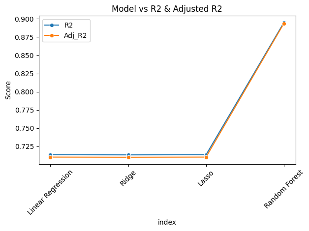
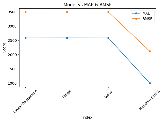
- From the above analysis, Random Forest gives the best R2 and Adj_R2 score. So we will use this model for deployment.
import joblib

final_model = RandomForestRegressor(random_state=42)
final_model.fit(X_train, y_train)

joblib.dump(final_model, "premium_model.pkl")
Overall Insights 💡
👉 Older - Obese and overweight people are got higher premium price.
👉 Younger - Normal and underweight people are got lower premium price.
👉 Those people have gone for any transplants surgery, got the higher premium price.
👉 People who are more than 60years old have gone through 3 major surgeries. And their premium prices are same 28K.
👉 For 2 major surgeries, around the age of 50 to 60 years old, their premium amount is also same 28K.
👉 Age and premium price are highly co-related.
👉 From the statistical test, except the Known Allergies all other Diabetes, Blood pressure, Transplants, Chronic diseases and History of Cancer in Family have significant difference in Premium Price, which means they are the factors impacting the premium price.
👉 Both BMI and Age groups have significant impact on the premium price.
👉 Except the known allergies, then the rest are have significant association with the Premium price.