Delivery Time Prediction
Problem Statement
- To train a regression model to predict the estimated delivery time.
Importing Python Libraries
import numpy as np
import pandas as pd
import matplotlib.pyplot as plt
import seaborn as sns

import warnings
warnings.filterwarnings('ignore')
Loading the Dataset
df = pd.read_csv("data.csv")
Data Exploration (EDA)
df.shape
df.head(5)
df.info()
df.describe()
df.isnull().sum()
💡 Observation
- There are no null values present in the data set.
# Converting the features to date time format

df['created_at'] = pd.to_datetime(df['created_at'])
df['actual_delivery_time'] = pd.to_datetime(df['actual_delivery_time'])
cols = df.columns

for col in cols:
    print(f"{col}:", df[col].nunique())
cols = df[['market_id', 'order_protocol']]

for col in cols:
    print(df[col].value_counts())
# Creating the Target feature "estimated_minutes"

df['estimated_time'] = df['actual_delivery_time'] - df['created_at']
df['estimated_minutes'] = (df['estimated_time'].dt.total_seconds() // 60).astype('Int64')
df['estimated_minutes'].describe()
💡 Observation
- From the given data, the minimum time for the delivery is $32$ minutes and the maximum time for the delivery is $110$ minutes.
- And average time of around ~$46$ minutes.
# Outlier detection

def outlier_det(data, col):
    q1 = data[col].quantile(0.25)
    q3 = data[col].quantile(0.75)
    iqr = q3 - q1
    lower_bound = q1-(1.5*iqr)
    upper_bound = q3+(1.5*iqr)

    outliers = (data[col] < lower_bound) | (data[col] > upper_bound)
    count = int(outliers.sum())
    percent = round((count/data.shape[0]) * 100, 2)
    print(f"{col}:\n{count} outliers ({percent}%)\n")

    return outliers
columns = df.select_dtypes(include=np.number).columns.tolist()

for col in columns:
    outlier_det(df, col)
# Outlier treatment

def iqr_cap(df, cols=None, k=1.5, round_int_bounds=True):
    if cols is None:
        cols = df.select_dtypes(include=np.number).columns
    capped = df.copy()
    for c in cols:
        s = capped[c]
        q1 = capped[c].quantile(0.25)
        q3 = capped[c].quantile(0.75)
        iqr = q3 - q1
        low = q1 - k * iqr
        up  = q3 + k * iqr

        if pd.api.types.is_integer_dtype(s.dtype):

            if round_int_bounds:
                low_i = int(np.floor(low))
                up_i  = int(np.ceil(up))
                capped[c] = s.clip(lower=low_i, upper=up_i)
            else:

                capped[c] = s.astype(float).clip(lower=low, upper=up).round().astype(s.dtype)
        else:
            capped[c] = s.clip(lower=low, upper=up)

    return capped
df1 = iqr_cap(df, k=1.5)
Visual Analysis
plt.figure(figsize=(10,6))
sns.histplot(data=df1, x='estimated_minutes', kde=True)
plt.show()
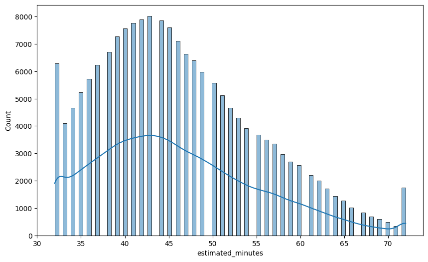
💡Observation
- The target feature, estimated minutes is right skewed.
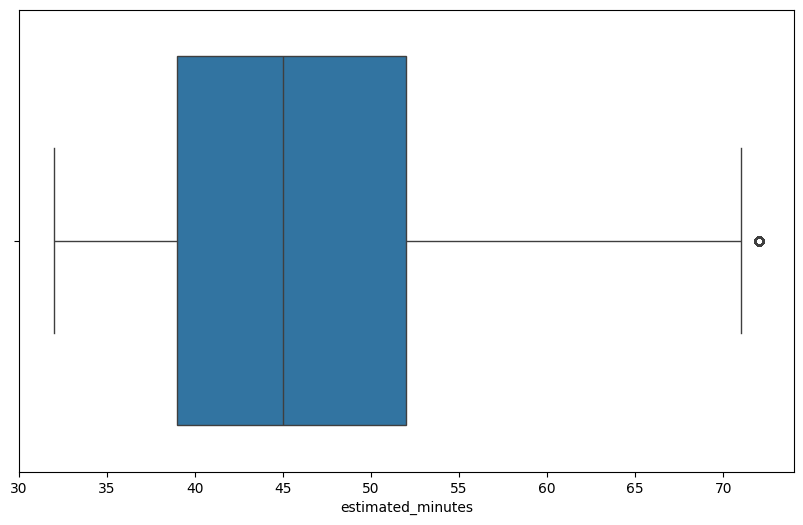
plt.figure(figsize=(10,6))
sns.boxplot(data=df1, x='estimated_minutes')
plt.show()
df1["created_date"] = df1["created_at"].dt.strftime("%Y-%m-%d")
df1["created_time"] = df1["created_at"].dt.strftime("%H:%M:%S")
df1["delivered_date"] = df1["actual_delivery_time"].dt.strftime("%Y-%m-%d")
df1["delivered_time"] = df1["actual_delivery_time"].dt.strftime("%H:%M:%S")
df1["actual_delivery_time"] = pd.to_datetime(df1["actual_delivery_time"], errors="coerce")

h = df1["actual_delivery_time"].dt.hour  # 0..23 [web:145]

# Shift hours so that 21->0, 22->1, 23->2, 0->3, ... 20->23
h_shift = (h - 21) % 24  # wrap-around via modulo [web:146]

# Define bins on shifted scale:
# 0 -> night:    0–8   (maps to 21:00–04:59)
# 1 -> morning:  9–15  (05:00–11:59)
# 2 -> afternoon:16–20 (12:00–16:59)
# 3 -> evening:  21–23 (17:00–20:59)
bins   = [-0.1, 9, 16, 21, 24]
labels = [0, 1, 2, 3]

df1["delivery_session"] = pd.cut(
    h_shift, bins=bins, labels=labels, right=False, include_lowest=True
)
# If week day then 1 else if weekend then 0

df1["created_on"]  = np.where(df1["created_at"].dt.weekday < 5, 1, 0)
df1["delivered_on"] = np.where(df1["actual_delivery_time"].dt.weekday < 5, 1, 0)
df1_corr = df1.corr('spearman', numeric_only=True)

plt.figure(figsize=(9, 6))
sns.heatmap(df1_corr, annot=True, cmap='coolwarm', fmt = '.2f', linewidths=0.5)
plt.show()
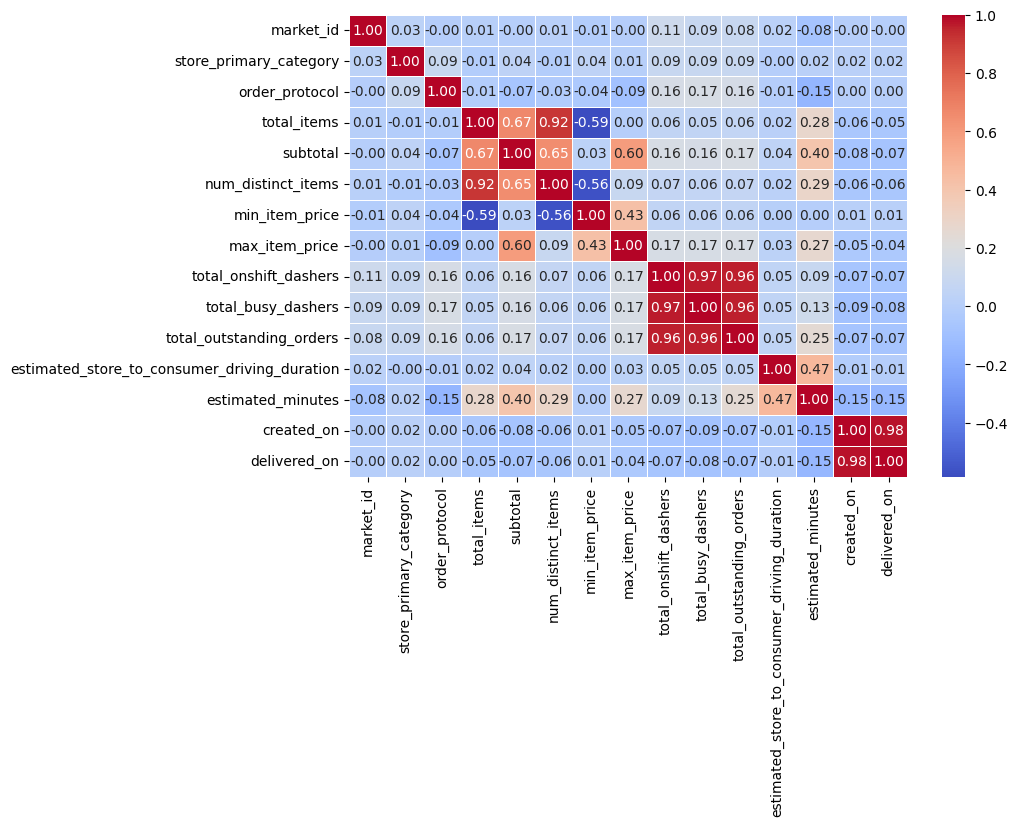
💡Observation
- From the above correlation heat map, the following features are highly correlated.
- Number of distinct items vs total items → quite obivious, because of the number of items.
- The features → total_onshift_dashers, total_busy_dashers, total_outstanding_orders are also highly correlated.
# Prep counts
left_ct = df1.groupby(['created_on','delivery_session']).size().unstack(fill_value=0).sort_index()
right_ct = df1.groupby(['delivered_on','delivery_session']).size().unstack(fill_value=0).sort_index()

def stacked_bar(ax, ct, title, xlab):
    bottoms = None
    colors = plt.cm.tab10(np.linspace(0, 1, ct.shape[1]))
    for (col, color) in zip(ct.columns, colors):
        ax.bar(ct.index, ct[col], bottom=bottoms, label=col, color=color, width=0.6)
        bottoms = (ct[col] if bottoms is None else bottoms + ct[col])
    ax.set_title(title)
    ax.set_xlabel(xlab)
    ax.set_ylabel('count')
    ax.legend(title='delivery_session')

plt.figure(figsize=(9,6))
ax1 = plt.subplot(1,2,1)
stacked_bar(ax1, left_ct, 'Number of orders created', 'created_on')

ax2 = plt.subplot(1,2,2)
stacked_bar(ax2, right_ct, 'Number of orders delivered', 'delivered_on')

plt.tight_layout()
plt.show()
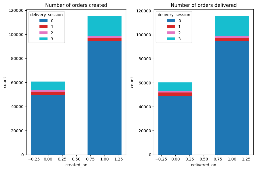
💡 Observation
The majority of the orders placed during the weekdays. And all the orders are delivered in the same day. But there is a small discrepancy because if someone placed order during Friday before midnight then the order delivered after midnight which is technically the next day (saturday) and vice versa.
Also most of the orders were placed during night and evening time.
| Label | Session | Day |
|---|---|---|
| 0 | Night | Weekend |
| 1 | Morning | Weekday |
| 2 | Afternoon | - |
| 3 | Evening | - |
avg_os = df1.groupby(['created_on','delivery_session'])['total_outstanding_orders'].mean().unstack(fill_value=0).sort_index()
avg_busy = df1.groupby(['created_on','delivery_session'])['total_busy_dashers'].mean().unstack(fill_value=0).sort_index()
avg_os_das = df1.groupby(['created_on','delivery_session'])['total_onshift_dashers'].mean().unstack(fill_value=0).sort_index()

def stacked_bar(ax, ct, title, xlab):
    bottoms = None
    colors = plt.cm.tab10(np.linspace(0, 1, ct.shape[1]))
    for (col, color) in zip(ct.columns, colors):
        ax.bar(ct.index.astype(str), ct[col].values, bottom=bottoms,
               label=f'session {col}', color=color, width=0.6)
        bottoms = ct[col].values if bottoms is None else bottoms + ct[col].values
    ax.set_title(title)
    ax.set_xlabel(xlab)
    ax.set_ylabel('average')
    ax.legend(title='delivery_session')

plt.figure(figsize=(12, 8))
ax1 = plt.subplot(1, 3, 1)
stacked_bar(ax1, avg_os, 'Avg. Outstanding Orders', 'created_on')

ax2 = plt.subplot(1, 3, 2)
stacked_bar(ax2, avg_busy, 'Avg. Busy Partners', 'created_on')

ax3 = plt.subplot(1, 3, 3)
stacked_bar(ax3, avg_os_das, 'Avg. Onshift Partners', 'created_on')

plt.tight_layout()
plt.show()
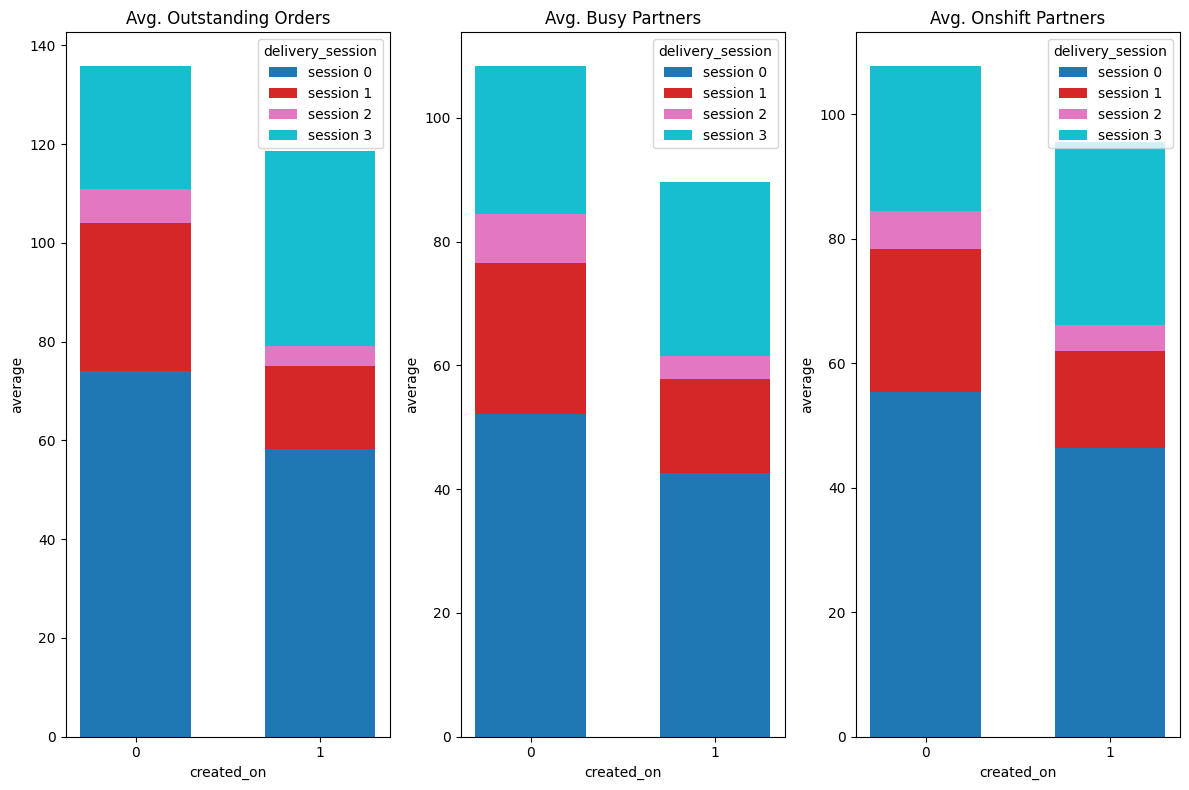
💡Observation
- The average outstanding orders, average busy dashers and average onshift dashers are more in the sessions morning, evening and night.
avg_os = df1.groupby('market_id')['total_outstanding_orders'].mean().sort_index().to_frame('avg_outstanding')
avg_busy = df1.groupby('market_id')['total_busy_dashers'].mean().sort_index().to_frame('avg_busy')
avg_os_das = df1.groupby('market_id')['total_onshift_dashers'].mean().sort_index().to_frame('avg_onshift')

def stacked_bar(ax, ct, title, xlab):
    bottoms = None
    colors = plt.cm.tab10(np.linspace(0, 1, ct.shape[1]))
    for (col, color) in zip(ct.columns, colors):
        ax.bar(ct.index.astype(str), ct[col].values,
               bottom=bottoms, label=col, color=color, width=0.6)
        bottoms = ct[col].values if bottoms is None else bottoms + ct[col].values
    ax.set_title(title)
    ax.set_xlabel('Market ID')
    ax.set_ylabel('Average')

plt.figure(figsize=(14, 6))

ax1 = plt.subplot(1, 3, 1)
stacked_bar(ax1, avg_os, 'Avg. Outstanding Orders', 'market_id')

ax2 = plt.subplot(1, 3, 2)
stacked_bar(ax2, avg_busy, 'Avg. Busy Partners', 'market_id')

ax3 = plt.subplot(1, 3, 3)
stacked_bar(ax3, avg_os_das, 'Avg. Onshift Partners', 'market_id')

plt.tight_layout()
plt.show()
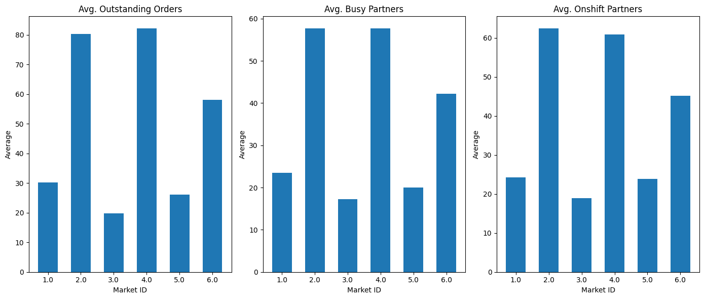
💡Observation
- The average outstanding orders, average busy dashers and average onshift dashers are more from the markets 2, 4 & 6.
counts = df1['market_id'].value_counts().sort_values(ascending=False)

plt.figure(figsize=(10,6))
ax = sns.barplot(
    x=counts.index.astype(str),  # cast to string to keep exact order
    y=counts.values,
    order=counts.index.astype(str),  # ensure order is enforced
    palette='viridis'
)

for bar, value in zip(ax.patches, counts.values):
    x = bar.get_x() + bar.get_width() / 2
    y = bar.get_height()
    ax.text(x, y + (0.01 * y), f"{value:,}",
            ha='center', va='bottom', fontsize=10)

plt.xlabel("Market ID")
plt.ylabel("Number of orders placed")
plt.title("Orders per Market ID")
plt.show()
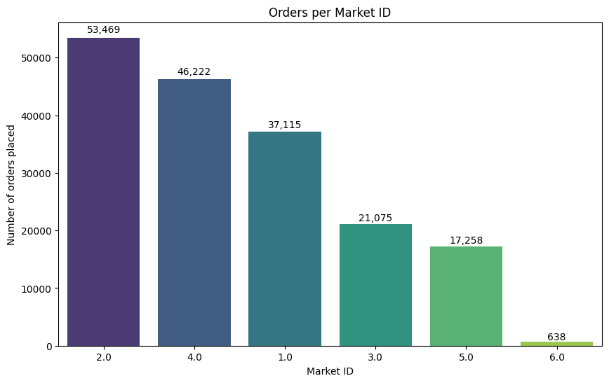
💡Observation
- From the above chart, most of the orders are placed from the Market 2 & 4.
- Market 6 has only very few orders.
counts = df1['order_protocol'].value_counts().sort_values(ascending=False)

plt.figure(figsize=(10,6))
ax = sns.barplot(
    x=counts.index.astype(str),  # cast to string to keep exact order
    y=counts.values,
    order=counts.index.astype(str),  # ensure order is enforced
    palette='viridis'
)

for bar, value in zip(ax.patches, counts.values):
    x = bar.get_x() + bar.get_width() / 2
    y = bar.get_height()
    ax.text(x, y + (0.01 * y), f"{value:,}",
            ha='center', va='bottom', fontsize=10)

plt.xlabel("Order Protocol")
plt.ylabel("Number of orders placed")
plt.title("Orders per Order protocol")
plt.show()
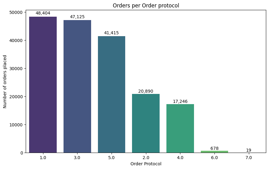
💡Observation
- From the above chart, most of the orders are placed in 1, 3 & 5.
- Only very few orders placed in 6 & 7.
cols = ['order_protocol', 'market_id', 'created_on', 'delivery_session']

fig, axes = plt.subplots(1, 4, figsize=(20, 4), sharey=True)

for ax, col in zip(axes, cols):
    avg_min = df1.groupby(col)['estimated_minutes'].mean().sort_index()
    ax.plot(avg_min, marker='o', color='steelblue')
    ax.set_xlabel(col)
    ax.set_title(f'{col} vs Avg. estimated minutes')

axes[0].set_ylabel('Average estimated minutes')

plt.tight_layout()
plt.show()
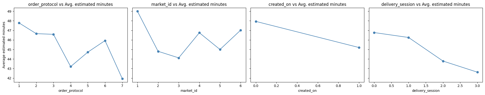
💡Observation
Strong influence of order protocol
- Some protocols inherently take longer → operational review needed.
Market variations are large
- Market 1 has high delivery time.
Estimated delivery time is lower in week days
Delivery sessions later in day are faster
Statistical Analysis
import statsmodels.api as sm
import statsmodels.formula.api as smf
from scipy import stats
from scipy.stats import kruskal
import scikit_posthocs as sp
df1['_log_dm'] = np.log(df1['estimated_minutes'].clip(lower=1e-6))
model_log = smf.ols('_log_dm ~ C(delivery_session)', data=df1).fit()
print(sm.stats.anova_lm(model_log, typ=2))
sm.stats.diagnostic.het_breuschpagan(model_log.resid,
                                     model_log.model.exog)
fig = sm.qqplot(df1['_log_dm'].dropna(), line='45')
plt.title('Q-Q plot of _log_dm')
plt.show()
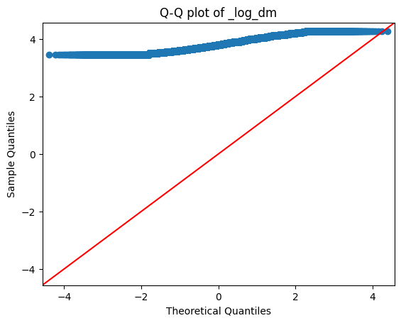
fig = sm.qqplot(df1['estimated_minutes'].dropna(), line='45')
plt.title('Q-Q plot of _log_dm')
plt.show()
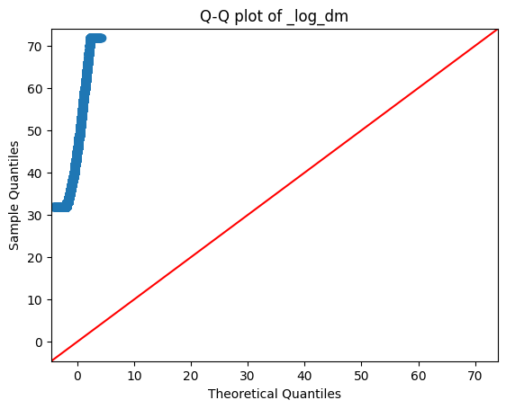
- The target column 'estimated minutes' is not normally distributed. Even after log transformations also it is still not normally distributed.
- Hence, we will use Kruskal-Wallis (non-parametric) test for our statistical analysis.
Kruskal - Wallis Test
- Null Hypothesis (H0): All groups come from the same distribution (i.e., their population medians are equal)
- Alternate Hypothesis (H1): At least one group has a different median → groups are not from the same distribution.
Target variable (estimated minutes) vs Order created
weekday_data = df1[df1['created_on'] == 0]['estimated_minutes']
weekend_data = df1[df1['created_on'] == 1]['estimated_minutes']

stat, p = kruskal(weekday_data, weekend_data)

print("Kruskal-Wallis Test: Weekday vs Weekend")
print("Statistic:", stat)
print("p-value:", p)

alpha = 0.05

if alpha < p:
    print('Fail to reject the null hypothesis. All groups come from the same distribution.')
else:
    print('Reject the null hypothesis. At least one group has significantly different median → groups are not from the same distribution.')
posthoc = sp.posthoc_dunn([weekday_data, weekend_data], p_adjust='bonferroni')

posthoc.index = ["weekday_data", "weekend_data"]
posthoc.columns = ["weekday_data", "weekend_data"]

print("Post-hoc Dunn Test (Weekday vs Weekend)")
print(posthoc)
💡Observation
- From the above 2 analysis, estimated delivery time differ between the weekday and weekend.
Target variable (estimated minutes) vs Session of the day
groups = []
labels = ["Night", "Morning", "Afternoon", "Evening"]
for s in [0, 1, 2, 3]:
    arr = df1[df1['delivery_session'] == s]['estimated_minutes'].astype(float).to_numpy()
    groups.append(arr)

stat, p = kruskal(*groups)

print("Kruskal-Wallis Test: Different sessions of the day")
print("Statistic:", stat)
print("p-value:", p)

alpha = 0.05

if alpha < p:
    print('Fail to reject the null hypothesis. All groups come from the same distribution.')
else:
    print('Reject the null hypothesis. At least one group has a different median → groups are not from the same distribution.')
posthoc = sp.posthoc_dunn(groups, p_adjust='bonferroni')

posthoc.index = labels
posthoc.columns = labels

print("Post-hoc Dunn Test (Time of Day)")
print(posthoc)
💡Observation
- A Kruskal–Wallis test indicated a statistically significant difference in estimated delivery times across session-of-day groups $(p < 0.001)$.
- Dunn post-hoc comparisons with Bonferroni correction revealed:
- No significant difference between Night and Morning deliveries $(p = 1.0)$.
- Afternoon and Evening deliveries differ significantly from both Night and Morning $(p < 0.001)$.
- Afternoon and Evening also differ significantly from each other $(p < 0.001)$.
This suggests that delivery times during Afternoon and Evening are statistically distinct and likely higher, indicating systematic variation based on time of day.
Target variable (estimated minutes) vs Market ID
mgroups = []
labels = list(df1['market_id'].unique().astype(str))
for s in range (1, df1['market_id'].nunique()+1):
    arr = df1[df1['market_id'] == s]['estimated_minutes'].astype(float).to_numpy()
    mgroups.append(arr)

stat, p = kruskal(*mgroups)

print("Kruskal-Wallis Test: Different Market ID")
print("Statistic:", stat)
print("p-value:", p)

alpha = 0.05

if alpha < p:
    print('Fail to reject the null hypothesis. All groups come from the same distribution.')
else:
    print('Reject the null hypothesis. At least one group has a different median → groups are not from the same distribution.')
posthoc = sp.posthoc_dunn(mgroups, p_adjust='bonferroni')

posthoc.index = labels
posthoc.columns = labels

print("Post-hoc Dunn Test (Market ID)")
print(posthoc)
💡Observation
Market 4 vs Market 6
$p = 0.7818687$ → NOT significant
Conclusion: Market 4 and Market 6 are similar.
Market 1 vs All Others
Market 1 shows $p = 0$ for all comparisons except itself.
Conclusion: Market 1 is significantly different from Markets 2, 3, 4, 5, 6.
Market 2 vs:
Market 3 → $p = 0.00233$ → significant
Market 4 → $p ≈ 2e-232$ → highly significant
Market 5 → $p ≈ 3e-16$ → highly significant
Market 6 → $p ≈ 1e-11$ → significant
Conclusion: Market 2 differs significantly from all markets.
Market 3 vs:
Market 4 → $p ≈ 3.6e-179$ → highly significant
Market 5 → $p ≈ 2.4e-23$ → highly significant
Market 6 → $p ≈ 6e-14$ → highly significant
Conclusion: Market 3 differs from all except itself.
Market 4 vs:
Market 5 → $p ≈ 3.5e-49$ → highly significant
Market 5 vs Market 6
$p ≈ 2.6e-06$ → significant
Conclusion
Except for Market 4 and Market 6, every market pair shows a statistically significant difference.
This implies the estimated minutes varies strongly across most Markets.
Target variable (estimated minutes) vs Order Protocol
ogroups = []
olabels = list(df1['order_protocol'].unique().astype(str))
for s in range (1, df1['order_protocol'].nunique()+1):
    arr = df1[df1['order_protocol'] == s]['estimated_minutes'].astype(float).to_numpy()
    ogroups.append(arr)

stat, p = kruskal(*ogroups)

print("Kruskal-Wallis Test: Different Order Protocol")
print("Statistic:", stat)
print("p-value:", p)

alpha = 0.05

if alpha < p:
    print('Fail to reject the null hypothesis. All groups come from the same distribution.')
else:
    print('Reject the null hypothesis. At least one group has a different median → groups are not from the same distribution.')
posthoc = sp.posthoc_dunn(ogroups, p_adjust='bonferroni')

posthoc.index = olabels
posthoc.columns = olabels

print("Post-hoc Dunn Test (Order Protocols)")
print(posthoc)
💡Observation
Protocol 1, Protocol 4, and Protocol 5 stand out—they have very different outcomes.
Protocols 2, 3, and 6 behave almost the same.
Protocol 7 is the "neutral" protocol—it does not differ from any others.
Chi-Square Test
from scipy.stats import chi2_contingency
def run_chi_square(df1, col1, col2):
    alpha = 0.05
    print("*"*100)
    print(f"▶️ Chi-Square Test: {col1} vs {col2}")

    table = pd.crosstab(df1[col1], df1[col2])
    chi2, p, dof, expected = chi2_contingency(table)

    print("Contingency Table:")
    print(table)

    print("\nResults:")
    print(f"Chi-square statistic: {chi2:.4f}")
    print(f"Degrees of freedom: {dof}")
    print(f"p-value: {p:.6f}")

    if p < alpha:
        print(f"➡️ Reject H₀: Significant association between {col1} and {col2}\n")
    else:
        print(f"➡️ Fail to Reject H₀: No association between {col1} and {col2}\n")
Market ID vs Others
cols = ['created_on', 'delivery_session', 'order_protocol']
col1 = 'market_id'
for col2 in cols:
    run_chi_square(df1, col1, col2)
Order Protocol vs others
cols = ['created_on', 'delivery_session']
col1 = 'order_protocol'
for col2 in cols:
    run_chi_square(df1, col1, col2)
Created on vs Delivery session
run_chi_square(df1, 'created_on', 'delivery_session')
📌 Chi-Square Test Summary
Market ID vs Created On
Strong association found
Different markets show different order-creation patterns
Market ID vs Delivery Session
Significant relationship
Delivery session distribution varies across markets
Market ID vs Order Protocol
Very strong association
Order protocols differ heavily by market
Order Protocol vs Created On
Significant association
Order protocol usage changes between creation days (weekday(1) / weekend(0))
Order Protocol vs Delivery Session
Strong relationship
Different order protocols occur in different delivery sessions
Created On vs Delivery Session
Significant association
Delivery patterns differ between the two created_on groups
ML Devlopment
To predict delivery estimated minutes based on operational and market attributes.
This is a Supervised Regression problem.
from sklearn.model_selection import train_test_split, GridSearchCV, RandomizedSearchCV
from sklearn.preprocessing import StandardScaler
from sklearn.linear_model import LinearRegression
from sklearn.ensemble import RandomForestRegressor
from xgboost import XGBRegressor
import lightgbm as lgb
from sklearn.metrics import root_mean_squared_error, mean_absolute_error, r2_score
from statsmodels.stats.outliers_influence import variance_inflation_factor
Model Evalution
def model_evl(yt, yp):
    rmse = round(root_mean_squared_error(yt, yp), 4)
    mae = round(mean_absolute_error(yt, yp), 4)
    r2 = round(r2_score(yt, yp), 4)

    print(f"RMSE: {rmse}\nMAE: {mae}\nR2 score: {r2}")
Train Test Split
df1['created_date'] = pd.to_datetime(df1['created_date'])
df1['created_month'] = (df1['created_date']).dt.month
df1['created_year'] = (df1['created_date']).dt.year
df1['created_day'] = (df1['created_date']).dt.day_of_week

df1['delivered_date'] = pd.to_datetime(df1['delivered_date'])
df1['delivered_month'] = (df1['delivered_date']).dt.month
df1['delivered_year'] = (df1['delivered_date']).dt.year
df1['delivered_day'] = (df1['delivered_date']).dt.day_of_week
target = "estimated_minutes"
X = df1.drop(columns=[target, 'created_date', 'created_time', 'delivered_date', 'delivered_time',
                       'created_at', 'actual_delivery_time', 'estimated_time', "_log_dm"])

X['delivery_session'] = X['delivery_session'].astype(int)

y = df1[target]
X_train, X_test, y_train, y_test = train_test_split(X, y, test_size=0.2, random_state=42)
Tree Based Regression Models
Random Forest
rf = RandomForestRegressor(n_estimators=100, max_depth=30, random_state=42)

rf.fit(X_train, y_train)

y_pred = rf.predict(X_test)
val = rf.feature_importances_
val
columns = X.columns
fea_imp = pd.DataFrame(val).set_index(columns)
fea_imp.reset_index().sort_values(0, ascending=False)
X_dropped = X.drop(columns=['created_on', 'delivered_on', 'created_month', 'delivered_month', 'created_year', 'delivered_year'])
X_train_dropped, X_test_dropped, y_train, y_test = train_test_split(X_dropped, y, test_size=0.2, random_state=42)
rf.fit(X_train_dropped, y_train)

y_pred = rf.predict(X_test_dropped)
model_evl(y_pred, y_test)
# Predictions
train_pred = rf.predict(X_train)
test_pred = rf.predict(X_test)

# Train metrics
train_rmse = root_mean_squared_error(y_train, train_pred)
train_r2 = r2_score(y_train, train_pred)

# Test metrics
test_rmse = root_mean_squared_error(y_test, test_pred)
test_r2 = r2_score(y_test, test_pred)

print("=== Train Metrics ===")
print("Train RMSE:", train_rmse)
print("Train R2:", train_r2)

print("\n=== Test Metrics ===")
print("Test RMSE:", test_rmse)
print("Test R2:", test_r2)
result3 = model_evl(y_test, y_pred)
XGBoost
xgb = XGBRegressor(
    objective="reg:squarederror",
    eval_metric="rmse",
    tree_method="hist",
    n_jobs=-1,
    random_state=42
)

xgb.fit(X_train_dropped, y_train)

xgb_pred = xgb.predict(X_test_dropped)
# Predictions
train_pred = xgb.predict(X_train_dropped)
test_pred = xgb.predict(X_test_dropped)

# Train metrics
train_rmse = root_mean_squared_error(y_train, train_pred)
train_r2 = r2_score(y_train, train_pred)

# Test metrics
test_rmse = root_mean_squared_error(y_test, test_pred)
test_r2 = r2_score(y_test, test_pred)

print("=== Train Metrics ===")
print("Train RMSE:", train_rmse)
print("Train R2:", train_r2)

print("\n=== Test Metrics ===")
print("Test RMSE:", test_rmse)
print("Test R2:", test_r2)
r1 = model_evl(y_test, xgb_pred)
LightGBM
train_data = lgb.Dataset(X_train_dropped, label=y_train)
test_data = lgb.Dataset(X_test_dropped, label=y_test)
params = {
    'boosting_type': 'gbdt',
    'objective': 'regression',
    'metric': 'rmse',
    'learning_rate': 0.05,
    'min_data_in_leaf': 30,
    'num_leaves': 31,
    'max_depth': -1,
    'lambda_l1': 1.0,
    'lambda_l2': 1.0,
    'feature_fraction': 0.8,
    'bagging_fraction': 0.8,
    'bagging_freq': 5,
    'verbose': -1
}
model = lgb.train(
    params,
    train_data,
    valid_sets=[train_data, test_data],
    num_boost_round=9000
)
lgb_pred = model.predict(X_test_dropped, num_iteration=model.best_iteration)
# Predictions
train_pred = model.predict(X_train_dropped)
test_pred = model.predict(X_test_dropped)

# Train metrics
train_rmse = root_mean_squared_error(y_train, train_pred)
train_r2 = r2_score(y_train, train_pred)

# Test metrics
test_rmse =root_mean_squared_error(y_test, test_pred)
test_r2 = r2_score(y_test, test_pred)

print("=== Train Metrics ===")
print("Train RMSE:", train_rmse)
print("Train R2:", train_r2)

print("\n=== Test Metrics ===")
print("Test RMSE:", test_rmse)
print("Test R2:", test_r2)
lgb_score = model_evl(y_test, lgb_pred)
LGB for user interface
t = df1[df1['estimated_store_to_consumer_driving_duration'] == 861].head(3)
t[['estimated_store_to_consumer_driving_duration', 'estimated_minutes']]
X_train_new = X_train_dropped.drop(columns=['delivered_day'])
X_test_new = X_test_dropped.drop(columns=['delivered_day'])
train_data = lgb.Dataset(X_train_new, label=y_train)
test_data = lgb.Dataset(X_test_new, label=y_test)
model = lgb.train(
    params,
    train_data,
    valid_sets=[train_data, test_data],
    num_boost_round=9000
)
# Predictions
train_pred = model.predict(X_train_new)
test_pred = model.predict(X_test_new)

# Train metrics
train_rmse = root_mean_squared_error(y_train, train_pred)
train_r2 = r2_score(y_train, train_pred)

# Test metrics
test_rmse =root_mean_squared_error(y_test, test_pred)
test_r2 = r2_score(y_test, test_pred)

print("=== Train Metrics ===")
print("Train RMSE:", train_rmse)
print("Train R2:", train_r2)

print("\n=== Test Metrics ===")
print("Test RMSE:", test_rmse)
print("Test R2:", test_r2)
lgb_pred_u = model.predict(X_test_new, num_iteration=model.best_iteration)
lgb_score_u = model_evl(y_test, lgb_pred_u)
Linear Regression
VIF
def calculate_vif(df):
    vif_data = pd.DataFrame()
    vif_data["feature"] = df.columns
    vif_data["VIF"] = [variance_inflation_factor(df.values, i) for i in range(df.shape[1])]
    return vif_data
print("===== VIF BEFORE REMOVAL =====")
vif_before = calculate_vif(X)
print(vif_before)
# Remove features with VIF > 10
high_vif_cols = vif_before[vif_before["VIF"] > 10]["feature"].tolist()
X= X.drop(columns=high_vif_cols)

print("\nRemoved High-VIF Columns:", high_vif_cols)
print("===== VIF AFTER REMOVAL =====")
vif_after = calculate_vif(X)
print(vif_after)
Scaling
X = X.drop(columns=['created_year', 'delivered_year'])
scaler = StandardScaler()
X_scaled = scaler.fit_transform(X)
Xs_train, Xs_test, y_train, y_test = train_test_split(X_scaled, y, test_size=0.2, random_state=42)
Training
lr = LinearRegression()

lr.fit(Xs_train, y_train)

lr_pred = lr.predict(Xs_test)
model_evl(y_test, lr_pred)
✅ LightGBM Model – Final Summary for Deployment
Model Selected
The final model chosen for deployment is:
🎯LightGBM Regressor (Fine-Tuned Version)
LightGBM consistently delivered the best balance of accuracy, generalization, speed, and stability compared to Random Forest, XGBoost, and CatBoost.Reason for Choosing LightGBM
LightGBM was selected because:
 ✔ Highest test performance
     RMSE ≈ 1.27
     MAE ≈ 1.14
     R² ≈ 0.968

 ✔ Low overfitting (small gap between train & test metrics)

 ✔ Fast inference time, ideal for real-time predictions

 ✔ Handles:
     Large datasets efficiently
     High-cardinality categorical features
     Missing values
     Non-linear relationships

 ✔ Hyperparameters tune well and improve generalization
Final Model Performance
Train Metrics
RMSE: ~0.986
R²: ~0.9887Test Metrics
RMSE: ~1.27
R²: ~0.968These metrics indicate excellent predictive power.
import pickle

with open("lightgbm_model.pkl", "wb") as f:
    pickle.dump(model, f)
model.save_model("lightgbm_model.txt")
Neural Network Implementation
from sklearn.compose import ColumnTransformer
from sklearn.pipeline import Pipeline
from tensorflow.keras.models import Sequential
from tensorflow.keras.layers import Dense, Dropout
from tensorflow.keras.callbacks import EarlyStopping, ReduceLROnPlateau
import tensorflow as tf
from tensorflow import keras
from tensorflow.keras import layers
from keras.callbacks import EarlyStopping
import keras_tuner as kt
X.info()
X_dropped = X.drop(columns=['created_on', 'delivered_on'])
X_train_dropped, X_test_dropped, y_train, y_test = train_test_split(X_dropped, y, test_size=0.2, random_state=42)
scaler = StandardScaler()

scaler = StandardScaler()
scaler.fit(X_train_dropped)

X_train_scaled = scaler.transform(X_train_dropped)
X_test_scaled = scaler.transform(X_test_dropped)
X_train_scaled = X_train_scaled.astype("float32")
y_train = y_train.astype("float32")
model = Sequential([
    Dense(128, activation='relu', input_dim=X_train_scaled.shape[1]),
    Dropout(0.2),
    Dense(64, activation='relu'),
    Dense(32, activation='relu'),
    Dense(1)
])
model.compile(optimizer=tf.keras.optimizers.Adam(learning_rate=0.001),
              loss='mse',
              metrics=['mae'])
X_test_scaled = scaler.transform(X_test_dropped)
X_test_scaled = X_test_scaled.astype("float32")
y_test = y_test.astype("float32")
loss, mae = model.evaluate(X_test_scaled, y_test)
print("Test MAE:", mae)
print("Test RMSE:", loss**0.5)
def build_model(hp):
    model = keras.Sequential()

    # Input layer
    model.add(layers.Input(shape=(X_train_scaled.shape[1],)))

    # Number of layers
    for i in range(hp.Int("num_layers", 2, 5)):
        model.add(layers.Dense(
            units=hp.Int(f"units_{i}", min_value=64, max_value=512, step=64),
            activation="relu",
            kernel_initializer="he_normal"
        ))
        model.add(layers.BatchNormalization())
        model.add(layers.Dropout(hp.Float(f"dropout_{i}", 0.1, 0.4, step=0.1)))

    # Output (regression)
    model.add(layers.Dense(1))

    # Choose LR
    lr = hp.Float("lr", 1e-4, 5e-3, sampling="log")

    model.compile(
        optimizer=keras.optimizers.Adam(learning_rate=lr),
        loss="mse",
        metrics=["mae"]
    )

    return model
tuner = kt.RandomSearch(
    build_model,
    objective="val_mae",
    max_trials=10,
    executions_per_trial=1,
    directory="tuner_results",
    project_name="porter_nn"
)
tuner.search(
    X_train_scaled,
    y_train,
    validation_split=0.2,
    epochs=30,
    batch_size=32,
    callbacks=[
        EarlyStopping(monitor="val_loss", patience=10, restore_best_weights=True)
    ],
    verbose=1
)
best_model = tuner.get_best_models(num_models=1)[0]
Train Best Model Longer With LR Scheduler
es = EarlyStopping(monitor="val_loss", patience=15, restore_best_weights=True)
lr_reduce = ReduceLROnPlateau(monitor="val_loss", factor=0.5, patience=5)

history = best_model.fit(
    X_train_scaled,
    y_train,
    validation_split=0.2,
    epochs=200,
    batch_size=32,
    callbacks=[es, lr_reduce],
    verbose=1
)
X_test_scaled
y_pred = best_model.predict(X_test_scaled)
model_evl(y_pred, y_test)
best_model.save("best_lighting_nn.h5")
Summary
Final scores:
| Metric | NN Score | Light GBM Score |
|---|---|---|
| RMSE | 2.1281 | 1.27 |
| MAE | 1.56 | 1.14 |
| R² score | 0.94 | 0.968 |
- From the above comparisons, $Light GBM$ is performing better than $NN$. Hence we choose $Light GBM$ model for the final deployment.
- $NN$ scores compartively less, this could be due to the dataset size.