Scaler Clustering
Problem statement
Objective
- The objective of this project is to cluster Scaler learners based on their company, job position, experience, and compensation (CTC) to identify homogeneous groups with similar professional and salary characteristics.
- Both manual clustering (business-rule based) and unsupervised learning techniques (K-Means and Hierarchical Clustering) are applied to:
- Identify high-earning and low-earning learners
- Benchmark salaries across companies and roles
- Provide actionable insights to learners and Scaler’s business team
Import Libraries & Load Data
!pip install kneed
import pandas as pd
import numpy as np

import matplotlib.pyplot as plt
import seaborn as sns

import re
from datetime import datetime

from sklearn.preprocessing import StandardScaler, OneHotEncoder, LabelEncoder, MinMaxScaler
from sklearn.impute import SimpleImputer, KNNImputer
from sklearn.compose import ColumnTransformer
from sklearn.pipeline import Pipeline

from sklearn.cluster import KMeans, DBSCAN
from scipy.cluster.hierarchy import dendrogram, linkage
from sklearn.metrics import silhouette_score
from sklearn.utils import resample
from sklearn.mixture import GaussianMixture
from sklearn.cluster import AgglomerativeClustering

import warnings
warnings.filterwarnings('ignore')

from scipy.stats import kruskal, spearmanr, pearsonr, mannwhitneyu

from kneed import KneeLocator
!gdown 1Sg45aJZsKNEZdOSjJ5BnNoPhpBgyQf0L
df = pd.read_csv('/content/scaler_clustering.csv')
Basic EDA
Preliminary analysis
df.shape
df.info()
df.describe(include='all')
👁️ Observation
- Dataset contains both categorical (Company, Job_position) and numerical (CTC, orgyear) variables
- Email_hash and Company_hash are anonymized identifiers
- Unnamed: 0 is an index column → can be dropped
df.drop(columns=['Unnamed: 0'], inplace=True)
Unique Email Analysis
df['email_hash'].nunique()
df['email_hash'].value_counts().head(10)
👁️ Observation
- Multiple records for the same email indicate job switches, promotions, or salary updates.
- This justifies clustering at the learner-record level, not unique learner level.
CTC checking
df['ctc'].describe()
df['ctc'].min(), df['ctc'].max()
df[df['ctc'] < 200]
CTC is stored in mixed units:
- Some values are in lakhs (2, 6, 14, 15)
- Some values are in thousands (200, 600, 1000)
- Some are in actual amounts (1,000,000+)
Standardizing CTC
a = set(df['ctc'].unique())
a
def convert_ctc_to_lpa(ctc):
    """
    Converts CTC into Lakhs Per Annum (LPA)
    """

    if pd.isna(ctc):
        return np.nan

    # Monthly salary → convert to annual
    if ctc < 100000:
        annual_ctc = ctc * 12

    # Annual salary
    elif ctc <= 50000000:
        annual_ctc = ctc

    # Unrealistic values → mark as NaN
    else:
        return np.nan

    # Convert to LPA
    return annual_ctc / 100000


df['ctc_lpa'] = df['ctc'].apply(convert_ctc_to_lpa)
During EDA, observed that the raw CTC values were recorded in inconsistent units (monthly and annual), so we standardized them into Lakhs Per Annum using domain-driven rules before performing any outlier analysis or clustering.
Missing Values Handling (Mean / KNN Imputation)
df.isnull().sum()
Strategy:
Numerical → Mean or KNN Imputation
Categorical → Most frequent
num_cols = ['ctc_lpa', 'orgyear', 'ctc_updated_year']
cat_cols = ['company_hash', 'job_position']
num_imputer = KNNImputer(n_neighbors=5)
cat_imputer = SimpleImputer(strategy='most_frequent')

df[num_cols] = num_imputer.fit_transform(df[num_cols])
df[cat_cols] = cat_imputer.fit_transform(df[cat_cols])
Checking the years
invalid_years = df[df['ctc_updated_year'] < df['orgyear']]
invalid_years.shape
invalid_years.sample(5)
👁️ Observation
- Some records have CTC updated year earlier than organization joining year, which is logically inconsistent and indicates data quality issues.
- Let assume salary update happened at joining.
df['ctc_updated_year'] = np.where(
    df['ctc_updated_year'] < df['orgyear'],
    df['orgyear'],
    df['ctc_updated_year']
)
We observed records where ctc_updated_year was earlier than orgyear, which is logically inconsistent. To maintain data integrity, we corrected such cases by ensuring that the CTC updated year is not earlier than the joining year.
invalid_years = df[df['ctc_updated_year'] < df['orgyear']]
invalid_years.shape
Regex Cleaning (Company & Job Position)
def clean_text(text):
    return re.sub('[^A-Za-z0-9 ]+', '', str(text)).strip()

df['company_hash'] = df['company_hash'].apply(clean_text)
df['job_position'] = df['job_position'].apply(clean_text)
- Regex removes tabs, special characters, and inconsistent naming issues.
df['job_position_clean'] = (df['job_position'].str.lower().str.strip())
df['job_position_clean'].unique()
def map_job_category(title):
    if pd.isna(title) or title in ['', 'na', 'null', 'no', 'not applicable']:
        return 'Other / Non-Tech'

    title = title.lower()

    # Data roles
    if any(x in title for x in [
        'data scientist', 'data analyst', 'data engineer',
        'machine learning', 'ml', 'ai', 'analytics', 'applied scientist'
    ]):
        return 'Data'

    # Software engineering roles
    if any(x in title for x in [
        'software engineer', 'developer', 'sde', 'full stack',
        'backend', 'frontend', 'android', 'ios', 'mobile',
        'web developer', 'programmer', 'fullstack'
    ]):
        return 'Software Engineer'

    # QA / Testing
    if any(x in title for x in [
        'qa', 'test engineer', 'testing', 'sdet', 'automation'
    ]):
        return 'QA / Testing'

    # DevOps / Infra
    if any(x in title for x in [
        'devops', 'sre', 'site reliability', 'cloud',
        'platform engineer', 'infra', 'network'
    ]):
        return 'DevOps / Infra'

    # Product / Management
    if any(x in title for x in [
        'product manager', 'program manager', 'manager',
        'lead', 'director', 'head', 'cto', 'vp', 'architect'
    ]):
        return 'Product / Program / Manager'

    # Design roles
    if any(x in title for x in [
        'designer', 'ui', 'ux'
    ]):
        return 'Design'

    # Intern / Student
    if any(x in title for x in [
        'intern', 'trainee', 'student', 'apprentice', 'graduate'
    ]):
        return 'Intern / Student'

    # Business / Ops / Support
    if any(x in title for x in [
        'business', 'operations', 'support', 'consultant',
        'analyst', 'sales', 'marketing', 'hr'
    ]):
        return 'Business / Operations / Support'

    return 'Other / Non-Tech'
df['job_category'] = df['job_position_clean'].apply(map_job_category)
df['job_category'].value_counts()
df[df['job_position']=='Other'].shape[0]
df[df['job_category'] == 'Other / Non-Tech'].sample(5)
Duplicate Handling
df.duplicated().sum()
df.drop_duplicates(inplace=True)
org_rows = df.shape[0]
df.shape
Feature Engineering – Years of Experience
df['years_of_exp'] = df['ctc_updated_year'] - df['orgyear']

df['years_of_exp'].describe()
df[df['years_of_exp'] == 2021]
df[df['years_of_exp'] == -18146]
df[(df['orgyear'] > 2025) | (df['orgyear'] < 1970)].sample(10)
- From the above it seems that there is an error in the org year. We will remove these by doing outlier treatment.
Outlier treatment
def outlier_treatment(data, col):
    q1 = data[col].quantile(0.25)
    q3 = data[col].quantile(0.75)
    iqr = q3-q1

    lb = q1 - (1.5*iqr)
    ub = q3 + (1.5*iqr)

    outliers = data[(data[col]<lb) | (data[col]>ub)]

    print(f"Column: {col}")
    print(f"Lower Bound: {lb}")
    print(f"Upper Bound: {ub}")
    print(f"Number of outliers: {outliers.shape[0]}")
    print("\nOutliers:")
    print(outliers)
def remove_outliers(data, col):
    q1 = data[col].quantile(0.25)
    q3 = data[col].quantile(0.75)
    iqr = q3 - q1

    lb = q1 - 1.5 * iqr
    ub = q3 + 1.5 * iqr

    before = data.shape[0]

    data = data[(data[col] >= lb) & (data[col] <= ub)]

    after = data.shape[0]

    print(f"Number of rows before removal from {col}: {before}")
    print(f"Outliers removed from {col}: {before - after}")
    print(f"Number of rows after removal from {col}: {after}\n")
    return data
for col in num_cols:
    outlier_treatment(df, col)
for col in ['orgyear', 'ctc_updated_year']:
    df = remove_outliers(df, col)
# For CTC we will cap the outliers instead of removing them.
def cap_outliers(data, col):
    q1 = data[col].quantile(0.25)
    q3 = data[col].quantile(0.75)
    iqr = q3 - q1

    lb = q1 - 1.5 * iqr
    ub = q3 + 1.5 * iqr

    data[col] = np.clip(data[col], lb, ub)
    return data

df = cap_outliers(df, 'ctc_lpa')
rows_after_clean = df.shape[0]

print(f"Percentage of data removed after outlier removal: {round((org_rows-rows_after_clean)/org_rows *100, 2)}%")
Manual Clustering
Company + Job + Experience CTC Summary
df.info()
summary_cje = (
    df.groupby(['company_hash', 'job_position', 'years_of_exp'])
      .agg(
          avg_ctc=('ctc', 'mean'),
          min_ctc=('ctc', 'min'),
          max_ctc=('ctc', 'max'),
          count=('ctc', 'count')
      )
      .reset_index()
)
df = df.merge(summary_cje,
              on=['company_hash', 'job_position', 'years_of_exp'],
              how='left')
df.sample(5)
Designation Flag
Logic
- 1 → Above average
- 2 → Around average
- 3 → Below average
def designation_flag(row):
    if row['ctc'] > row['avg_ctc']:
        return 1
    elif row['ctc'] < row['avg_ctc']:
        return 3
    else:
        return 2

df['Designation'] = df.apply(designation_flag, axis=1)
df.sample(5)
Designation 1 learners are outperformers within same role & experience.
Class Flag (Company + Job Position)
summary_cj = (
    df.groupby(['company_hash', 'job_position'])
      .agg(avg_ctc_class=('ctc', 'mean'))
      .reset_index()
)
df = df.merge(summary_cj, on=['company_hash', 'job_position'], how='left')
df['class'] = np.where(
    df['ctc'] > df['avg_ctc_class'], 1,
    np.where(df['ctc'] < df['avg_ctc_class'], 3, 2)
)
Tier Flag (Company Level)
summary_company = (
    df.groupby('company_hash')
      .agg(avg_ctc_company=('ctc', 'mean'))
      .reset_index()
)
df = df.merge(summary_company, on='company_hash', how='left')
df['Tier'] = np.where(
    df['ctc'] > df['avg_ctc_company'], 1,
    np.where(df['ctc'] < df['avg_ctc_company'], 3, 2)
)
Visual Analysis
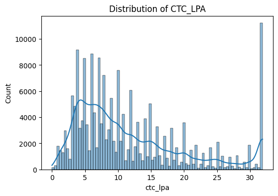
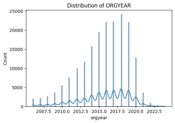
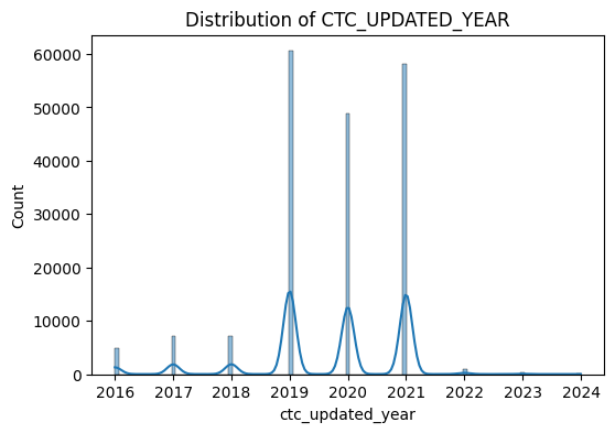
Univariate Analysis
for col in num_cols:
    plt.figure(figsize=(6,4))
    sns.histplot(df[col], kde=True)
    plt.title(f"Distribution of {col.upper()}")
    plt.show()
for col in num_cols:
    plt.figure(figsize=(6,4))
    sns.boxplot(y=df[col])
    plt.title(f"Boxplot of {col.upper()}")
    plt.show()
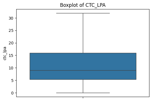
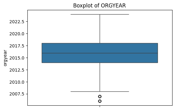
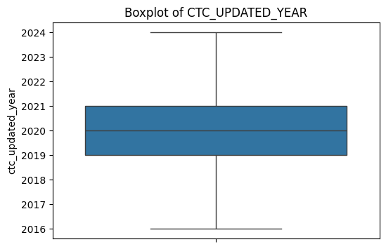
“CTC is right-skewed”
“Outliers significantly reduced after cleaning”
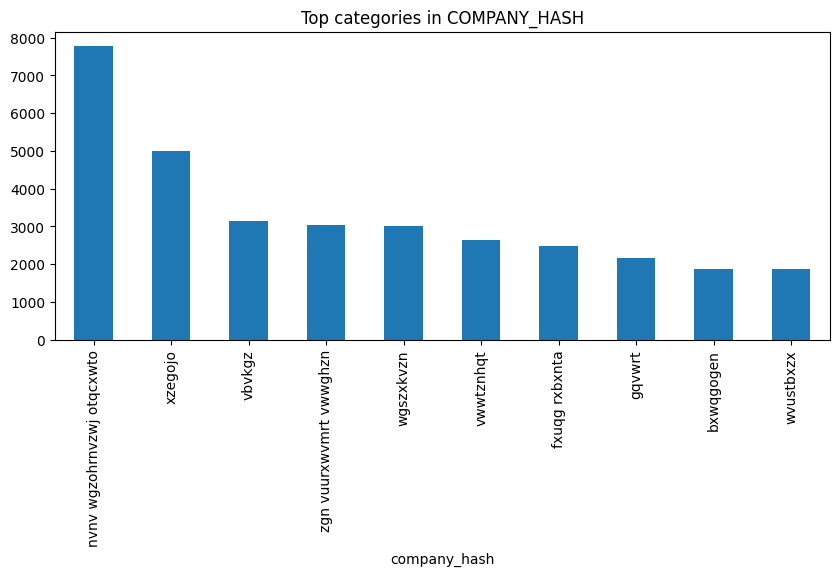
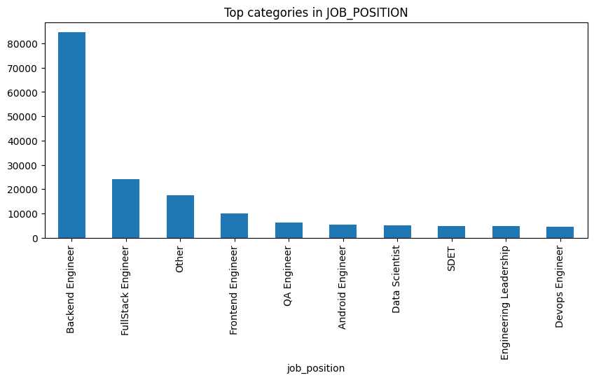
Categorical Variable Analysis
for col in cat_cols:
    plt.figure(figsize=(10,4))
    df[col].value_counts().head(10).plot(kind='bar')
    plt.title(f"Top categories in {col.upper()}")
    plt.show()
Bivariate Analysis
CTC vs Experience
plt.figure(figsize=(12,6))
sns.boxplot(x=round(df['years_of_exp']), y='ctc_lpa', data=df)
plt.xticks(rotation=45)
plt.title('CTC Distribution by Years of Experience')
plt.ylabel('CTC LPA')
plt.xlabel('Years of Experience')
plt.show()
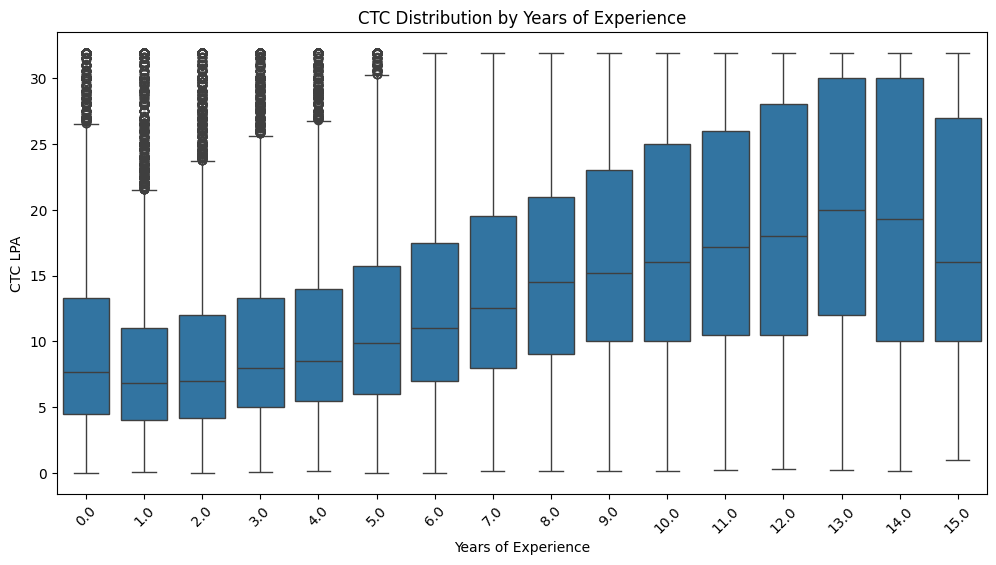
CTC increases with experience, but the widening salary spread and presence of high outliers across all experience levels indicate that role and company significantly influence compensation, making clustering a suitable approach.
CTC vs Job position
plt.figure(figsize=(12,6))
sns.boxplot(x='job_category', y='ctc_lpa', data=df)
plt.xticks(rotation=45)
plt.title('CTC Distribution by Job position')
plt.ylabel('CTC LPA')
plt.xlabel('Job position')
plt.show()
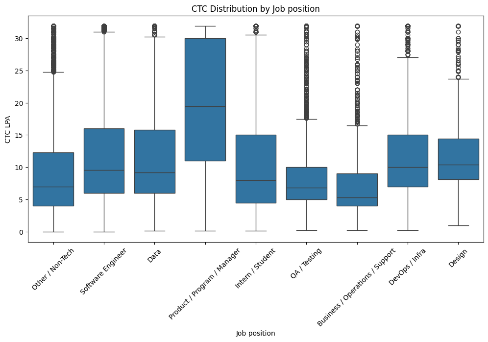
Product / Program / Manager roles command the highest median CTC, while Intern/Student and Business/Operations roles earn the lowest, with Software Engineering and DevOps showing strong but more variable pay growth.
Top 10 employees (Tier 1)
df[df['Tier'] == 1].sort_values('ctc_lpa', ascending=False).head(10)
Bottom 10 employees (Tier 3)
df[df['Tier'] == 3].sort_values('ctc_lpa').head(10)
Top 10 Data Science employees per company
df[
    (df['job_position'].str.contains('Data', case=False)) &
    (df['class'] == 1)
].sort_values('ctc', ascending=False).groupby('company_hash').head(10)
Top 10 Companies by CTC
df.groupby('company_hash')['ctc'].mean().sort_values(ascending=False).head(10)
Top 2 Positions per Company
df.groupby(['company_hash', 'job_position'])['ctc'].mean() \
  .reset_index() \
  .sort_values(['company_hash', 'ctc'], ascending=[True, False]) \
  .groupby('company_hash').head(2)
Across companies, technical roles such as Backend and Full-Stack Engineering consistently appear among the top two highest-paying positions based on average CTC.
Statistical Analysis
Normality test
from scipy.stats import shapiro

sample_ctc = df['ctc_lpa'].sample(5000, random_state=42)
stat, p = shapiro(sample_ctc)

if p < 0.05:
    print(f"p-Value is {p}. Hence CTC is not normally distributed")
else:
    print(f"p-Value is {p}. Hence CTC is normally distributed")
Since CTC is not normally distributed, we will use non-parametric tests.
Kruskal–Wallis Test
alpha = 0.05
CTC vs Job position
Hypotheses:
- H₀: Median CTC is the same across job categories
- H₁: At least one category differs
groups = [
    group['ctc_lpa'].values
    for _, group in df.groupby('job_position')
]

stat, p = kruskal(*groups)

if p < alpha:
    print("Kruskal-Wallis p-value:", p)
    print("Salary differs significantly by job position")

else:
    print("Kruskal-Wallis p-value:", p)
    print("No significant difference")
- CTC differs significantly across job categories/positions, validating the visual salary gaps observed.
CTC vs Experience
corr, p = pearsonr(df['years_of_exp'], df['ctc_lpa'])

print("Pearson Correlation:", corr)
print("p-value:", p)
corr, p = spearmanr(df['years_of_exp'], df['ctc_lpa'])

print("Spearman Correlation:", corr)
print("p-value:", p)
There is a statistically significant positive relationship between experience and CTC.
Tiers vs Salary Distributions
tier_groups = [
    df[df['Tier'] == t]['ctc_lpa']
    for t in df['Tier'].unique()
]

stat, p = kruskal(*tier_groups)

if p < 0.05:
    print(f"p-Value is {p}. Salary distributions differ significantly across Tier groups.")
else:
    print(f"p-Value is {p}. Salary distributions not differ across Tier groups.")
Since CTC is highly skewed and non-normally distributed, non-parametric statistical tests were applied.
Kruskal–Wallis tests confirmed that salary distributions differ significantly across job categories and tier levels.
Spearman correlation showed a statistically significant positive relationship between years of experience and CTC.
These results validate the patterns observed during exploratory data analysis.
ML Development
Data Processing for Unsupervised Learning
df.sample(5)
company_le = LabelEncoder()
job_le = LabelEncoder()
scaler = MinMaxScaler()
df['company_enc'] = company_le.fit_transform(df['company_hash'])
df['job_enc'] = job_le.fit_transform(df['job_position_clean'])

df['ctc_scaled'] = scaler.fit_transform(df[['ctc_lpa']])

X = df[['company_enc', 'job_enc', 'ctc_scaled', 'years_of_exp']]
X.head(5)
Elbow Method
inertia = []
K = range(1, 11)

for k in K:
    kmeans = KMeans(n_clusters=k, random_state=42)
    kmeans.fit(X)
    inertia.append(kmeans.inertia_)
kneedle = KneeLocator(
    K,
    inertia,
    curve='convex',
    direction='decreasing'
)

elbow_k = kneedle.elbow
elbow_inertia = inertia[K.index(elbow_k)]
plt.plot(K, inertia, marker='o')
plt.xlabel("Number of clusters")
plt.ylabel("Inertia")
plt.title("Elbow Method")

plt.annotate(
    f'Elbow Point (K={elbow_k})',
    xy=(elbow_k, elbow_inertia),
    xytext=(elbow_k + 1, elbow_inertia + 30000),
    arrowprops=dict(facecolor='red', arrowstyle='->'),
    fontsize=10
)

plt.show()
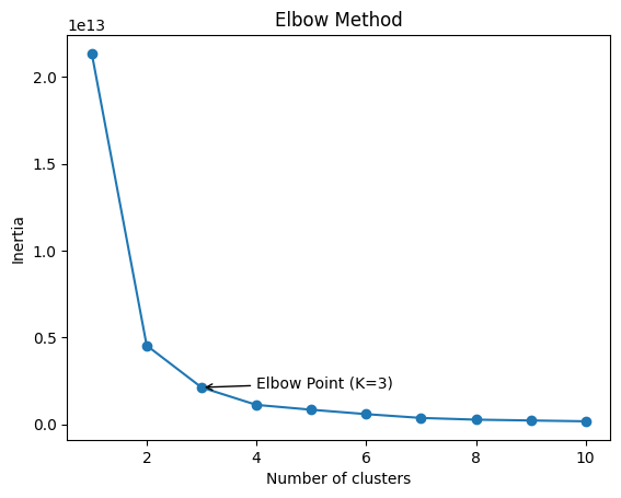
- We selected $K = 3$ because the inertia drops sharply up to $3$ clusters, after which the curve flattens.
- This indicates diminishing returns beyond $K = 3$, making it the optimal balance between cluster compactness and model simplicity.
ML Model
Silhouette score
def sil_score(x, labels, sample_frac=0.1, random_state=42):
    sample_size = int(0.1 * X.shape[0])
    X_sample, labels_sample = resample(
        x,
        labels,
        n_samples=sample_size,
        random_state=random_state,
        stratify=labels
    )

    score = silhouette_score(X_sample, labels_sample)

    return f"Silhouette Score (10% sample): {score:.4f}"
KMeans++
kmeans = KMeans(n_clusters=3, init='k-means++', random_state=42)

np.random.seed(45)
kmeans.fit(X)
klabels = kmeans.fit_predict(X)

sil_score(X, klabels)
X_km = X.copy()

X_km['klabels']=klabels

X_km.head(5)
Hierarchical Clustering (Sample)
np.random.seed(45)
sample = X[:1000]
linked = linkage(sample, method='ward')

plt.figure(figsize=(16, 6))
cut_height = 125000
plt.axhline(y=cut_height, color='red', linestyle='--', linewidth=1)
dendrogram(linked)
plt.show()

- Hierarchical clustering shows a clear separation into three major clusters when cut at distance $≈125,000$.
- These clusters likely represent low, medium, and high compensation groups, validating the KMeans result ($k=3$).
- The large vertical gaps indicate strong natural grouping in the data.
Agglomerative clustering
n_samples = int(0.1 * X.shape[0])
np.random.seed(42)
idx = np.random.choice(X.shape[0], size=n_samples, replace=False)

X_sample = X.iloc[idx]

model = AgglomerativeClustering(n_clusters=4, linkage='ward')

agg_labels = model.fit_predict(X_sample)
print(f"Agglomerative - Silhouette score: {round(silhouette_score(X_sample, agg_labels), 4)}")
X_sample_agg = X_sample.copy(deep=True)

X_sample_agg['agg_labels'] = agg_labels

X_sample_agg.head(5)
GMM (Gaussian Mixture Model)
X_gmm_sample = X_sample.copy(deep=True)
gmm = GaussianMixture(
    n_components=4,
    covariance_type='full',
    random_state=42
)
gmm_labels = gmm.fit_predict(X_gmm_sample)

sil = silhouette_score(X_gmm_sample, gmm_labels)
print(f"GMM Silhouette Score: {sil:.4f}")
X_gmm_sample['gmm_lables'] = gmm_labels

X_gmm_sample.head(5)
- GMM score is very low and seems very poor clustering of the data.
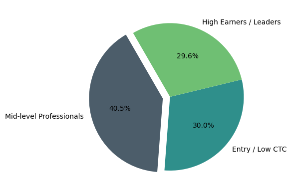
X_km['cluster'] = X_km['klabels'].map({0: 'Entry / Low CTC', 1: 'Mid-level Professionals', 2: 'High Earners / Leaders'})
chart = X_km['cluster'].value_counts().reset_index()
plt.pie(x=chart['count'],
        labels=chart['cluster'],
        explode = (0.1, 0, 0),
        colors = ['#4C5D6A', '#2F8F8B', '#6FBF73'],
        autopct='%1.1f%%',
        startangle=120)

plt.show()
📊 Business Recommendations
1. Compensation Benchmarking
Companies can use these clusters to:
- Compare their employee pay distribution against the market
- Identify overpaying or underpaying roles
➡️ Example: If most employees fall into Mid-level cluster but competitors place similar roles in High Earners, there is a retention risk.
2. Role-Based Salary Bands
HR teams should define salary bands by job position, not just experience.
✔ Recommended:
- Maintain role-specific salary ranges
- Adjust compensation policies based on market cluster positioning
3. Talent Retention & Career Planning
Employees can be mapped to clusters to:
- Identify high performers stuck in lower pay clusters
- Design promotion and upskilling paths to move employees upward
4. Hiring & Offer Strategy
For new hires:
- Predict likely cluster placement based on role + experience
- Make competitive but controlled offers aligned with market clusters
5. Strategic Workforce Planning
Leadership can use cluster insights to:
- Forecast payroll growth
- Plan leadership hiring
- Balance cost vs expertise across teams